Bayesian and frequentist inference for inverse problems in the presence of randomness.

Dyed-in-the-wool Bayesians like to talk about the decision theoretic benefits of being Bayesian. But I find it more convincing for myself and others to think of Bayesian inference as an approach to inverse problems in the presence of randomness.

During my PhD, a lot of my talks blended frequentist and Bayesian concepts, so I would often open the talk with the following animations to clarify the difference between the two approaches. Both frequentist and Bayesian approaches make sense. But, to first order, frequentist approaches are tailor-made for prediction problems, and Bayesian approaches are made for inference problems.

The inverse problem

Let us suppose we have positied a data generating model, which maps an unobserved parameter (\(\theta\)) to observed data (\(X\)). Call the probability distribution given by the generative model \(p(X | \theta)\). We observe \(X\) and want to know what \(\theta\) might be. If the map from \(\theta\) to \(X\) were invertible, there would be no difficulty. But we imagine that there is not a one-to-one map from \(\theta\) to \(X\) because of randomness.

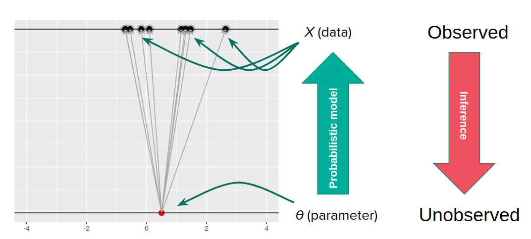
For my purposes here, we can imagine that there was one true \(\theta\) that generated the \(X\) we saw, we just don’t know what it was.

The frequentist approach

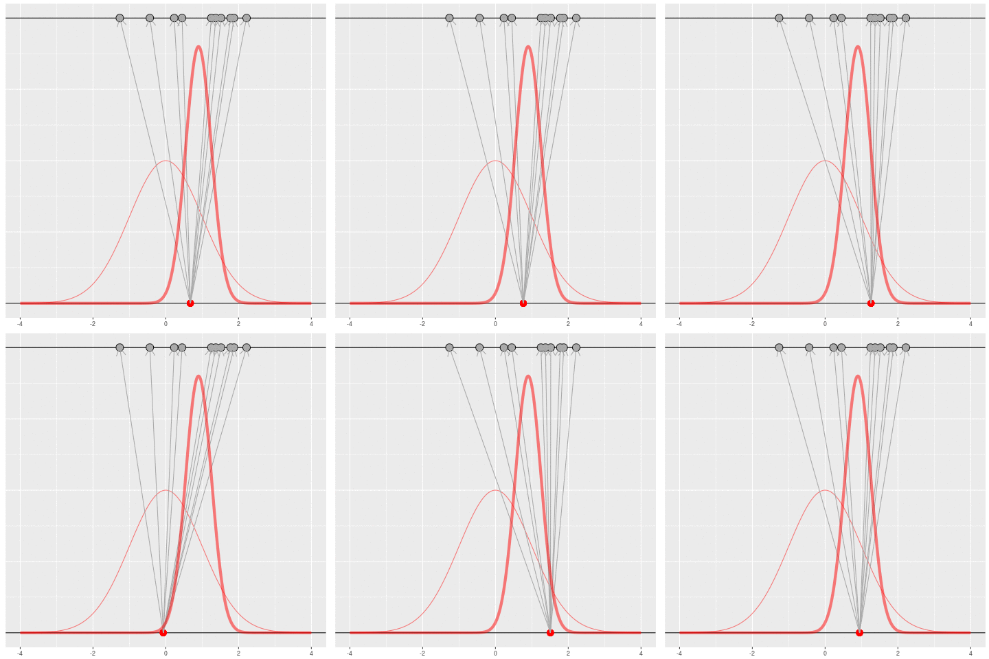
We got the parameter indicated by the red dot and saw the dataset in black. But, because of the randomness, the same parameter could have given us lots of other datasets.

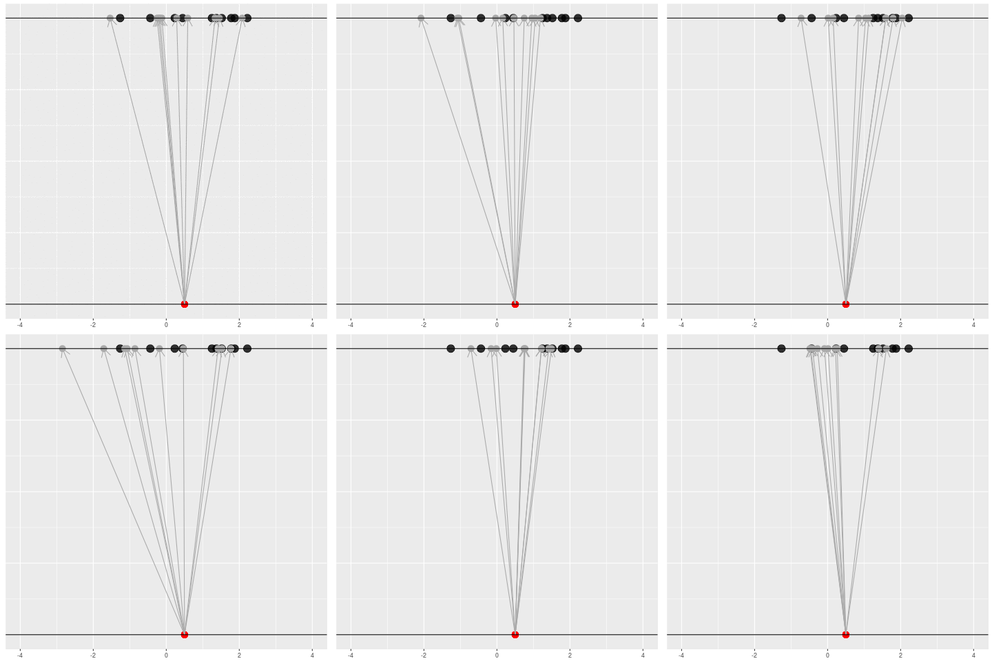
For each dataset, we might pick some summary function and call it an “estimate”. It will be different each time because the data will be different each time.

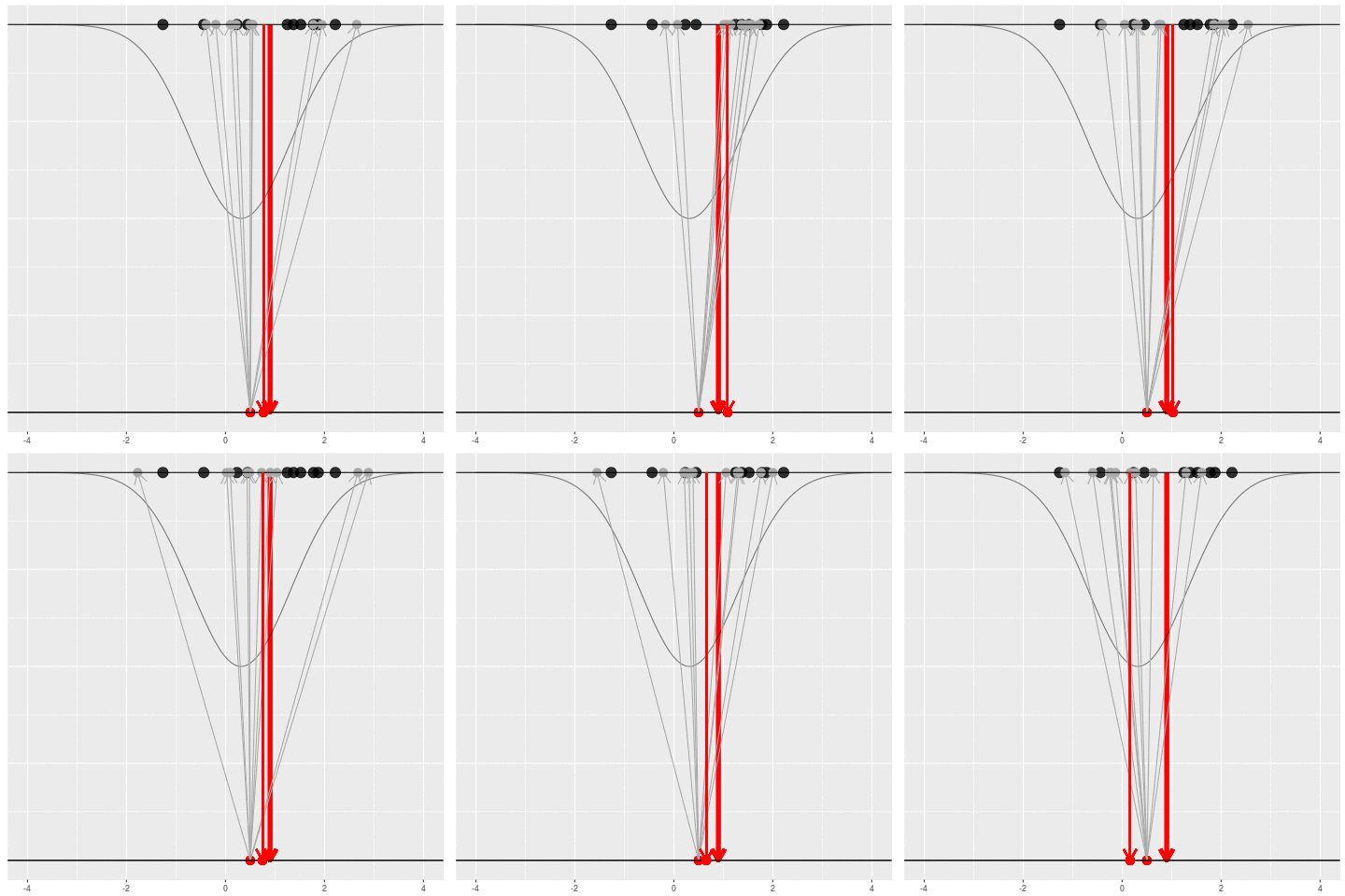
What can be an “estimate”? Technically, anything! But we hope the estimate we choose is usually near the true parameter in some sense. By “usually near”, we typically mean that it is unbiased, consistent, minimax, or some other criterion which we can guarantee without knowing \(\theta\) itself.

The Bayesian approach

Let’s imagine that the universe generates datasets by

• First drawing a parameter from some prior distribution…
• …and then drawing a dataset from that parameter.

Sometimes we would get the dataset we saw. Mostly we wouldn’t.

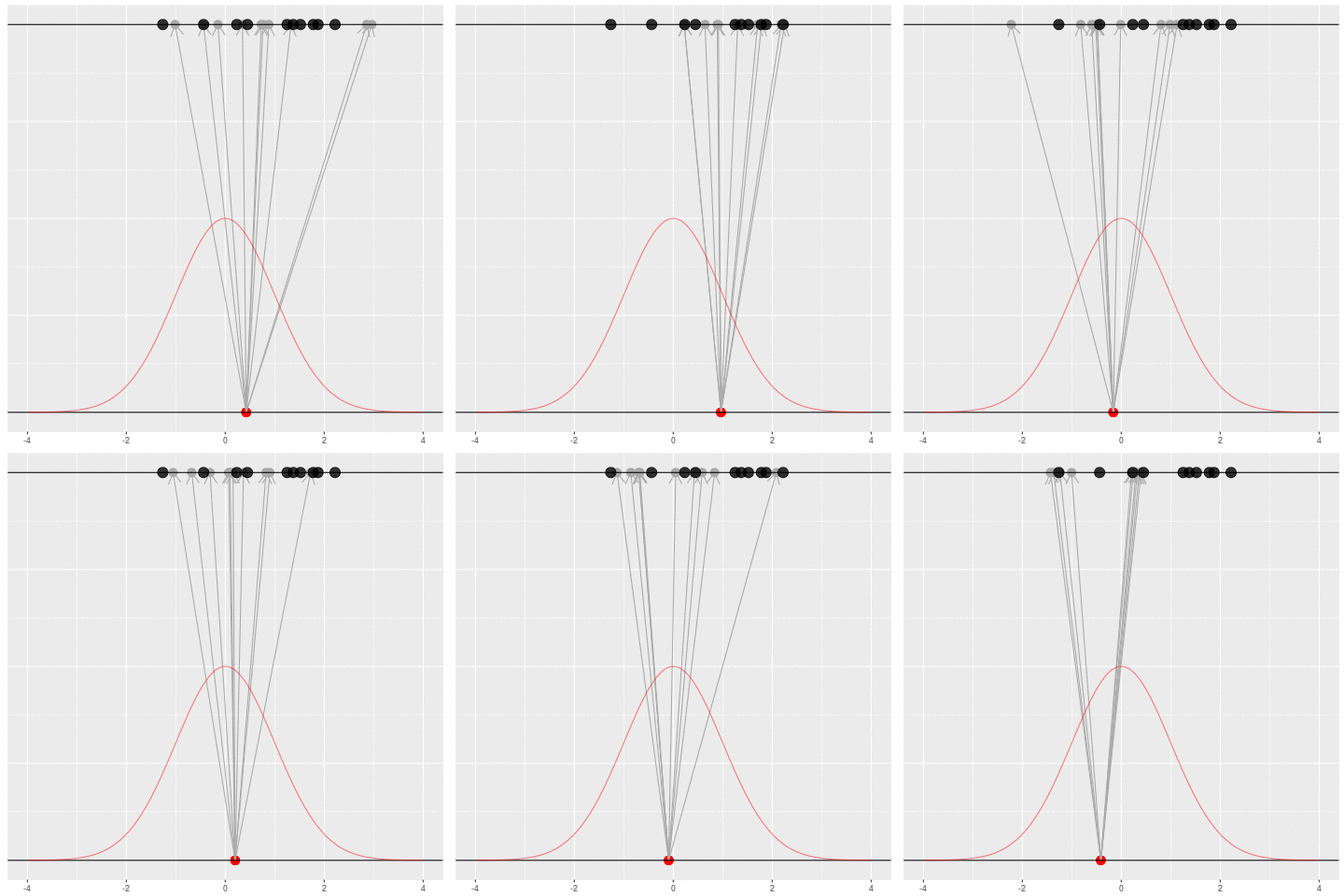
Suppose we draw a bunch of parameters and datasets pairs, and then throw out every pair where the data doesn’t match what we observed. (In theory, we can actually do this because we know the prior and the generative model.)

The distribution of the parameters that are left represents which parameters could have plausibly given us the dataset we saw. This distribution is called the “posterior” distribution. It’s the set of parameters left after repeating the generating process and keeping only \(X\) that matches the observations.

Of course, in practice you don’t usually generate parameters and data hoping to get your original dataset. That would be incredibly computationally intensive, because you would very rarely generate matches to the data you saw.

Instead, you use Bayes’ rule, which gives an analytic expression for the posterior \(p(\theta | X)\):

\[p(\theta | X) = \frac{p(X | \theta) p(\theta)}{p(X)}.\]

Bayes’ rule is an analytic description of the process of generating new datasets and throwing out the non-matches. But even this is intractable in general (the denominator is a problem). In practice, we turn to further approximation schemes like MCMC, Laplace approximations, variational Bayes, etc.

Comparison

• To perform frequentist inference:
  • We hope that our estimator tells us something about the true \(\theta\).
  • We hope that we can find the sampling distribution of the estimator even though we don’t know the true \(\theta\).
• To perform Bayesian inferene:
  • We hope the prior is reasonable and the data generating model is accurate.
  • We hope that we can somehow get an approximation of the posterior.

Both are approaches are reasonable and interesting, with different strengths and weaknesses! They are answering fundamentally different questions about the randomness you saw.

Frequentist	Bayesian