In the previous post, I introduced some notation and concepts that I’ll now carry forward into an actual sketch of how to prove the BCLT.

Recall that, for the BCLT we need to analyze quantites of the following form:

\[\mathbb{E}[\phi(\theta) | x] = \frac{\int \phi(\theta) \exp(\sum_{n=1}^N \ell(x_n | \theta)) \pi(\theta) d\theta} {\int \exp(\sum_{n=1}^N \ell(x_n | \theta)) \pi(\theta) d\theta}.\]

We may let \(\phi\) depend implicitly on \(N\), e.g., to evaluate functions of the form \(\phi(\sqrt{N}(\theta - \hat\theta))\), for example.

The argument will roughly proceed as follows.

First, we’ll form a Taylor series expansion of the log likelihood \(\sum_{n=1}^N \ell(x_n | \theta)\) and massage it into a form consisting of convergent quantities.
As part of the Taylor series expansion, we’ll define the re-scaled parameter \(\tau = \sqrt{N}(\theta - \hat\theta)\). We will be re-writing the posterior as an integral over \(\tau\).
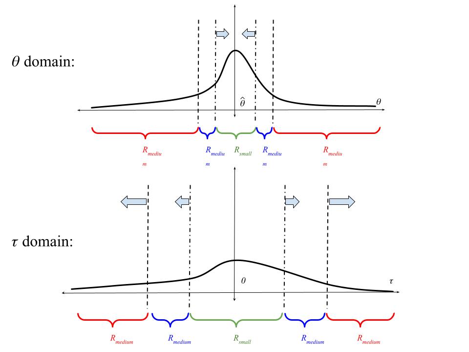
Next, we will divide the domain into three regions: \(R_{small}\), \(R_{medium}\), and \(R_{big}\), as shown in the following picture. We will specify the boundaries of these regions so that \(R_{small}\) shrinks in the domain of \(\theta\) but grows in the domain of \(\tau\) (i.e., after multiplication by \(\sqrt{N}\)).
We will show that we can choose the boundaries of the regions so that the contributions of \(R_{big}\) and \(R_{medium}\) are exponentially small in \(N\) under some moment conditions on \(\phi\). We will do this by:
- In region \(R_{big}\), by assuming that \(\hat\theta\) is a strict optimum and
- In region \(R_{medium}\), bounding the integral by a normal tail probability.
Thus, only region \(R_{small}\) makes a non-vanishing contribution to the posterior expectation, and in \(R_{small}\) we can reason just as we did for the MLE.


The BCLT divides the domain of integration up into these three regions. The arrows indicate what happens to the region boundary as \(N \rightarrow \infty\). Asymptotically, only the region \(R_{small}\) contributes to the posterior.

Re-write a posterior expectation as a random function that doesn’t diverge.

Recall that, to prove asymptotic normality of the MLE, we studied the asymptotic behavior of the Taylor expansion of the random log likelihood function,

\[\theta \mapsto \frac{1}{N} \sum_{n=1}^N \ell(x_n \vert \theta).\]

The factor of \(1/N\) in the MLE is a stark difference with the Bayesian case, as the posterior involves the random function

\[\theta \mapsto \sum_{n=1}^N \ell(x_n | \theta),\]

which diverges as \(N \rightarrow \infty\)! Before even beginning, we must re-write our expectation in a form involving something that looks like sample averages, not a divergent sum.

To do so, we’ll first write out our Taylor series expansion. For the moment, we’ll expand around a generic \(\bar\theta\).

\[\sum_{n=1}^N \ell(x_n | \theta) = \sum_{n=1}^N \ell(x_n | \bar\theta) + \sum_{n=1}^N \ell_{(1)}(x_n | \bar\theta)(\theta - \bar\theta) + \frac{1}{2}\sum_{n=1}^N \ell_{(2)}(x_n | \bar\theta)(\theta - \bar\theta)^2 + \frac{1}{6}\sum_{n=1}^N \ell_{(3)}(x_n | \tilde\theta)(\theta - \bar\theta)^3.\]

Here, the argument \(\tilde\theta\) to \(\ell_{(3)}(x_n | \tilde\theta)\) is somewhere in between \(\hat\theta\) and \(\theta\) as given by the mean value theorem.

At first glance, each term in the Taylor series still contains \(N\) terms, so it might not seem like we’ve gotten much. However, we expect to be able to choose \(\bar\theta\) so that, in regions that matter, \(|\theta - \bar\theta| = O(1 / \sqrt{N})\), so that higher powers of \(\theta - \bar\theta\) will decrease asymptotically.

So let’s try a parameterization that inflates \(\theta\) at the rate \(\sqrt{N}\). Specifically, for any \(\bar\theta\) depending only on the data, we can define the Bayesian parameter

\[\tau := \sqrt{N} (\theta - \bar\theta) \quad\quad \Leftrightarrow \quad \quad \theta = \frac{\tau}{\sqrt{N}} + \bar\theta.\]

Plugging in, we have

\[\sum_{n=1}^N \ell(x_n | \theta) = \sum_{n=1}^N \ell(x_n | \bar\theta) + \frac{1}{\sqrt{N}} \sum_{n=1}^N \ell_{(1)}(x_n | \bar\theta) \tau + \frac{1}{2} \frac{1}{N} \sum_{n=1}^N \ell_{(2)}(x_n | \bar\theta)\tau^2 + \frac{1}{6} \frac{1}{N^{3/2}} \sum_{n=1}^N \ell_{(3)}(x_n | \tilde\theta)\tau^3.\]

Note that in this new formula, the derivatives are still with respect to \(\theta\) — we’ve simply plugged \(\tau\) into the previous expression.

Now we’re getting somewhere, because the quadratic term looks like what we expect from a normal distribution, and the cubic term is a sample average times an additional power of \(1/\sqrt{N}\), and so goes to zero.

Two terms need to be dealt with. First, the term \(\frac{1}{\sqrt{N}} \sum_{n=1}^N \ell_{(1)}(x_n | \bar\theta) \tau\) is \(O_p(1)\) by an ordinary central limit theorem. Fortunately, we can get rid of this term by simply evaluating at \(\bar\theta = \hat\theta\), since then \(\sum_{n=1}^N \ell_{(1)}(x_n | \bar\theta)\) is identically zero by the first-order condition defining \(\hat\theta\). And, second, we observe that \(\sum_{n=1}^N \ell(x_n | \bar\theta)\) does not depend on \(\theta\), and so cancels in the numerator and denominator of \(\mathbb{E}[\phi(\theta) | x]\).

Before we plug into \(\mathbb{E}[\phi(\theta) | x]\), we need to deal with the effect of the change of variables on the prior. By the ordinary rules of density transformation, \(\pi(\theta) d\theta\) = \(\frac{1}{\sqrt{N} }\pi(\tau / \sqrt{N} + \hat\theta) d\tau\). Again, the factor of \(\frac{1}{\sqrt{N} }\) will cancel in the numerator and denominator. Putting all together, we get

\[\mathbb{E}[\phi(\theta) | x] = \frac{\int \phi(\tau / \sqrt{N} + \hat\theta) \exp\left( \frac{1}{2} \frac{1}{N} \sum_{n=1}^N \ell_{(2)}(x_n | \hat\theta)\tau^2 + \frac{1}{6} \frac{1}{N^{3/2}} \sum_{n=1}^N \ell_{(3)}(x_n | \tilde\theta)\tau^3 \right) \pi(\tau / \sqrt{N} + \hat\theta) d\tau} {\int \exp\left( \frac{1}{2} \frac{1}{N} \sum_{n=1}^N \ell_{(2)}(x_n | \hat\theta)\tau^2 + \frac{1}{6} \frac{1}{N^{3/2}} \sum_{n=1}^N \ell_{(3)}(x_n | \tilde\theta)\tau^3 \right) \pi(\tau / \sqrt{N} + \hat\theta) d\tau}.\]

We can now study \(\mathbb{E}[\phi(\theta) | x]\) by studying integrals of the following form, depending on some generic function \(\psi(\theta)\):

\[I(\psi) := \int \psi(\tau / \sqrt{N} + \hat\theta) \exp\left( \frac{1}{2} \left( \frac{1}{N} \sum_{n=1}^N \ell_{(2)}(x_n | \hat\theta) \right) \tau^2 + \frac{1}{6} \frac{1}{\sqrt{N}} \left( \frac{1}{N} \sum_{n=1}^N \ell_{(3)}(x_n | \tilde\theta) \right) \tau^3 \right) \pi(\tau / \sqrt{N} + \hat\theta) d\tau,\]

since \(\mathbb{E}[\phi(\theta) | x] = I(\phi) / I(1)\). Importantly, \(I(\psi)\) is an integral over quantities that will not diverge as \(N \rightarrow \infty\), and we have accomplished the goal of this first section.

The big region

Let’s now think about what sorts of problems we might have with \(I(\psi)\) for \(\theta\) (or, equivalently, \(\tau\)) in different regions of the real line. When \(N\) is large, then, by a ULLN applied to \(\ell_{(2)}(x_n | \theta)\),

\[\begin{align*} \frac{1}{N} \ell_{(2)}(x_n | \hat\theta) \approx -\mathcal{I}. \end{align*}\]

Can we hope to control \(\frac{1}{N} \sum_{n=1}^N \ell_{(3)}(x_n | \tilde\theta)\) by a ULLN in a similar way? Recall from the Taylor series that, for a given \(\theta\) (or, equivalently, a given \(\tau\)), all we know is that

\[\vert \tilde\theta - \hat\theta \vert \le \Big\vert \theta - \hat\theta \Big\vert \le \Big\vert \frac{\tau}{\sqrt{N}} \Big\vert.\]

And recall from the previous post that it is not reasonable to expect a ULLN to hold over unbounded domains. Consequently, we can only apply a ULLN to apply to \(\frac{1}{N} \sum_{n=1}^N \ell_{(3)}(x_n | \tilde\theta)\) for \(\theta\) in a fixed ball around \(\hat\theta\), or, equivalently, \(\tau\) in a domain that grows no faster than \(\sqrt{N}\). But, of course, for any \(N\), the integral \(I(\psi)\) also depends on values of \(\tau\) that are arbitrarily large. For such large \(\tau\) we must control \(I(\psi)\) some other way.

Consequently, we first consider the region

\[R_{big} = \left\{ \theta: |\theta - \hat\theta| > \delta_1 \right\},\]

for some \(\delta_1\). Equivalently, we can write

\[R_{big} = \left\{ \tau: |\tau| > \sqrt{N} \delta_1 \right\}.\]

Let \(I_{big}(\psi)\) denote the integral restricted to the region \(R_{big}\).

Within \(R_{big}\) our Taylor series is of no use, since we cannot control the \(\frac{1}{N} \sum_{n=1}^N \ell_{(3)}(x_n | \tilde\theta)\) term. However, we can plug the original function back into the Taylor series to write

\[\begin{align*} I_{big}(\psi) ={}& \int_{\tau \in R_{big}} \psi(\tau / \sqrt{N} + \hat\theta) \exp\left( \sum_{n=1}^N \ell(x_n | \tau / \sqrt{N} + \hat\theta) - \sum_{n=1}^N \ell(x_n | \hat\theta) \right) \pi(\tau / \sqrt{N} + \hat\theta) d\tau \\ ={}& \int_{\tau \in R_{big}} \psi(\tau / \sqrt{N} + \hat\theta) \exp\left( \sum_{n=1}^N \ell(x_n | \theta) - \sum_{n=1}^N \ell(x_n | \hat\theta) \right) \pi(\tau / \sqrt{N} + \hat\theta) d\tau. \end{align*}\]

One particularly simple way to control this integral is to assume that \(\hat\theta\) is a strict optimum of the data log likelihood, in the sense that, for any \(\delta_1\), there exists some \(\epsilon\) such that

\[\sup_{\theta \in R_{big}} \frac{1}{N} \sum_{n=1}^N \ell(x_n | \theta) - \frac{1}{N} \sum_{n=1}^N \ell(x_n | \hat\theta) < -\epsilon.\]

This condition will fail, for example, if the data log likelihood has multiple modes that are equally large. In such a case we surely wouldn’t expect a BCLT to hold. It will succeed if there is, with high probability, a single mode which is strictly above the rest of the log likelihood.

This is a strange condition, since it’s an assumption on the data, rather than on any population quantity. One would rather say that \(\mathbb{E}[ \ell(x_1 | \theta) ]\) has a strict optimum (where the expectation is over \(x_1\)), and that \(\frac{1}{N} \sum_{n=1}^N \ell(x_n | \theta)\) approach \(\mathbb{E}[ \ell(x_1 | \theta) ]\) sufficiently uniformly for all \(\theta\) such that \(\frac{1}{N} \sum_{n=1}^N \ell(x_n | \theta)\) inherits this property. But of course it is unreasonable to expect a ULLN to hold for all \(\theta \in R_{big}\). Some authors thus simply assume what is necessary (e.g., Chapter 6 of Theory of Point Estimation by Lehmann), and we will do the same. There is a more elegant but arguably less transparent solution to this region due to Le Cam, based on the existence of consistent tests. See chapter 10 of van Der Vaart’s Asymptotic Statistics for a discussion of this approach.

When we do have strict optimality,

\[\begin{align*} \vert I_{big}(\psi)\vert \le{}& \int_{\tau \in R_{big}} \vert\psi(\tau / \sqrt{N} + \hat\theta)\vert \exp\left( \sup_{\theta \in R_{big}} \sum_{n=1}^N \ell(x_n \vert \theta) - \sum_{n=1}^N \ell(x_n \vert \hat\theta) \right) \pi(\tau / \sqrt{N} + \hat\theta) d\tau \\ \le{}& \int_{\tau \in R_{big}} \vert\psi(\tau / \sqrt{N} + \hat\theta)\vert \exp\left( N \sup_{\theta \in R_{big}} \frac{1}{N} \sum_{n=1}^N \ell(x_n \vert \theta) - \frac{1}{N} \sum_{n=1}^N \ell(x_n \vert \hat\theta) \right) \pi(\tau / \sqrt{N} + \hat\theta) d\tau \\ \le{}& \exp\left(- N \epsilon\right) \int_{\theta \in R_{big}} \vert\psi(\theta)\vert \pi(\theta) d\theta. \end{align*}\]

Consequently, as long as \(\int \vert\psi(\theta)\vert \pi(\theta) d\theta\) is finite grows sub-exponentially in \(N\) — i.e., \(\mathbb{E}_{\pi}[\vert\psi(\theta)\vert] = o_p(\exp(N \epsilon))\) — then the contribution to \(I(\psi)\) from region \(R_{big}\) decays exponentially quickly in \(N\).

It’s worth mentioning before we go on that \(R_{big}\) is the only region in which we need to worry about the prior \(\pi(\theta)\) being proper, or the function \(\psi(\theta)\) being unbounded, since from now on we will be limiting ourselves to the ball \(\mathbb{R} \setminus R_{big}\).

Applying the ULLN and making everything look “Normal”

We now know that the contribution \(I_{big}(\psi)\) shrinks very quickly as \(N\) gets large, and outside the set \(R_{big}\), we can apply our ULLNs, so from now on let’s define

\[M_3 := \frac{1}{6} \mathbb{E}[ \ell_{(3)}(x_n \vert \theta_0)]\]

and work with

\[\begin{align*} I(\psi) \approx {}& \int_{\tau \in \mathbb{R} \setminus R_{big}} \psi(\tau / \sqrt{N} + \hat\theta) \exp\left( \left( -\frac{1}{2} \mathcal{I} + M_3 \frac{\tau}{\sqrt{N}} \right) \tau^2 \right) \pi(\tau / \sqrt{N} + \hat\theta) d\tau. \end{align*}\]

In the previous display I’ve pulled out a factor of \(\tau^2\), since that’s what we expect to be left with in a Normal density, but note that a \(\tau\) is still lurking inside the parenthesis. Dealing with that lurking \(\tau\) is the business that we now turn to.

The small region

Let’s take on the small, easy region: a shrinking ball in the domain of \(\theta\), centered at \(\hat\theta\). Within such a region we can hope to reason exactly as we did for the MLE.

Let’s take some real number \(\delta_2 > 0\) and define

\[R_{small} = \left\{ \theta: |\theta - \hat\theta| < \frac{\delta_2}{\log N} \right\}.\]

We can equivalently write

\[R_{small} = \left\{ \tau: |\tau| < \frac{\sqrt{N}}{\log N} \delta_2 \right\}.\]

As before, let \(I_{small}(\psi)\) denote \(I(\psi)\) restricted to the region \(R_{small}\). Note that, for any choices of \(\delta_1\) and \(\delta_2\), we eventually have \(R_{small} \subset \mathbb{R} \setminus R_{big}\), and we’ll assume without further comment that \(N\) is large enough that the sets nest in this way.

By letting \(R_{small}\) shrink at a rate \(1 / \log N\) in the \(\theta\) domain, we have defined a shrinking region in \(\theta\), but a growing region in \(\tau\). As far as our analysis of \(R_{small}\) is concerned, any set that shrinks in the domain of \(\theta\) but grows in the domain of \(\tau\) will do. For example, we might have had the region shrink at a rate \(\delta_2 / N^{1/4}\), but not \(\delta_2 / N\), since the latter would result in a region that shrunk in the domain of \(\tau\) as well. But for the middle region (which we will analyze next), the rate \(\log N\) will work out well.

Within \(R_{small}\), \(\vert \tau \vert \le \delta_2 \frac{\sqrt{N}}{\log N}\), so \(\vert \tau / \sqrt{N} \vert \le \frac{\delta_2}{\log N} \rightarrow 0\), and the lurking \(\tau\) term goes to zero at rate \(\log N\), and we can write

\[\begin{align*} I_{small}(\psi) \approx {}& %\int_{\tau \in R_{small}} %\psi(\tau / \sqrt{N} + \hat\theta) \exp\left( % \left( -\frac{1}{2} \mathcal{I} + % M_3 \frac{\delta_2}{\log N} % \right) \tau^2 %\right) % \pi(\tau / \sqrt{N} + \hat\theta) d\tau %\\ \approx {}& \int_{\tau \in R_{small}} \exp\left( -\frac{1}{2} \mathcal{I} \tau^2 \right) \psi(\tau / \sqrt{N} + \hat\theta) \pi(\tau / \sqrt{N} + \hat\theta) d\tau. \end{align*}\]

Furthermore, using the fact that \(\pi\) is continuous, we can write

\[\pi(\tau / \sqrt{N} + \hat\theta) = \pi(\hat\theta) + O_p(N^{-1/2}).\]

Also taking into account the fact that \(R_{small}\) grows in the \(\tau\) domain as \(N \rightarrow \infty\), this is nearly what we want — a Gaussian integral over the whole domain:

\[\begin{align*} I_{small}(\psi) \approx {}& \int \exp\left( -\frac{1}{2} \mathcal{I} \tau^2 \right) \psi(\tau / \sqrt{N} + \hat\theta) \pi(\hat\theta) d\tau. \end{align*}\]

But we still must deal with the contribution from the region we’ve left out, the gap between \(R_{small}\) and \(R_{big}\).

The medium region

We still have to analyze the region in between \(R_{small}\) and \(R_{big}\), which we call \(R_{medium}\):

\[R_{medium} = \left\{ \theta: \frac{\delta_2}{\log N} \le |\theta - \hat\theta| \le \delta_1 \right\},\]

or equivalently

\[R_{medium} = \left\{ \tau: \frac{\sqrt{N}}{\log N} \delta_2 \le |\tau| \le \sqrt{N} \delta_1 \right\}.\]

Here, the lurking \(\tau\) does not automatically go to zero, since we may have \(\tau\) as large as \(|\tau| / \sqrt{N} \le \delta_1\). However, we are free to choose \(\delta_1\), and we know that \(\mathcal{I}\) is positive. So we can choose \(\delta_1\) small enough that the quantity

\[\sup_{\tau \in R_{med}} \left( -\frac{1}{2} \mathcal{I} + M_3 \frac{\tau}{\sqrt{N}} \right) \le -\frac{1}{2} \mathcal{I} + M_3 \delta_1\]

is negative. For example, we could take \(\delta_1 = \frac{1}{4} \mathcal{I} / M_3\) to get \(\sup_{\tau \in R_{med}} \left( -\frac{1}{2} \mathcal{I} + M_3 \frac{\tau}{\sqrt{N}} \right) \le -\frac{1}{4} \mathcal{I}.\)

With this choice of \(\delta_1\), the restriction \(I_{medium}(\psi)\) of \(I(\psi)\) to \(R_{medium}\) is bounded above by a Gaussian integral:

\[\begin{align*} \vert I_{medium}(\psi) \vert \le{}& \int_{\tau \in R_{medium}} \exp\left( -\frac{1}{4} \mathcal{I} \tau^2 \right) \vert \psi(\tau / \sqrt{N} + \hat\theta) \vert \pi(\tau / \sqrt{N} + \hat\theta) d\tau \\\le{}& \int_{\tau: \vert \tau \vert \ge \frac{\sqrt{N}}{\log N} \delta_2} \exp\left( -\frac{1}{4} \mathcal{I} \tau^2 \right) \vert \psi(\tau / \sqrt{N} + \hat\theta) \vert \pi(\tau / \sqrt{N} + \hat\theta) d\tau. \end{align*}\]

In the last line we ignore the fact that \(R_{medium}\) is bounded above in the integral, though recall we have already used the fact that it is bounded above to make sure the term inside the exponent was negative.

We now see that \(I_{medium}(\psi)\) is controlled by the tail integral of a Gaussian density. The prior term doesn’t matter, since we know that \(\sup_{\tau \in R_{medium}} \pi(\tau / \sqrt{N} + \hat\theta) = \sup_{\theta \in R_{medium}} \pi(\theta) < \infty\) as long as the prior density is continuous. As long as the function \(\vert \psi(\tau / \sqrt{N} + \hat\theta) \vert\) is well behaved under the distribution \(\tau \sim \mathcal{N}(\tau \vert 0, \mathcal{I} / 2))\), then we can make \(I_{medium}(\psi)\) go to zero at any rate we like by choosing \(\delta_2\) sufficiently large, as we now illustrate.

For some constant \(C\) which accounts for both the prior and the normalizing constant of the Gaussian distribution, then, by Cauchy-Schwartz, we can re-write the preceding display as

\[\begin{align*} \vert I_{medium}(\psi) \vert \le{}& C \cdot \mathbb{E}_{\mathcal{N}(\tau \vert 0, \mathcal{I} / 2))} \left[ \vert \psi(\tau / \sqrt{N} + \hat\theta) \vert 1\left(\vert \tau \vert \ge \frac{\sqrt{N}}{\log N} \delta_2 \right) \right] \\\le{}& C \cdot \mathbb{E}_{\mathcal{N}(\tau \vert 0, \mathcal{I} / 2))} \left[ \vert \psi(\tau / \sqrt{N} + \hat\theta) \vert^2 \right]^{1/2} \mathbb{E}_{\mathcal{N}(\tau \vert 0, \mathcal{I} / 2))} \left[ 1\left(\vert \tau \vert \ge \frac{\sqrt{N}}{\log N} \delta_2 \right) \right]^{1/2}. \end{align*}\]

The final term is a Gaussian tail probability, which decays very quickly as \(\frac{\sqrt{N}}{\log N} \delta_2\) gets large. For example, we can write

\[\begin{align*} \int \exp\left( -\frac{1}{4} \mathcal{I} \tau^2 \right) 1\left(\vert \tau \vert \ge \frac{\sqrt{N}}{\log N} \delta_2 \right) d \tau ={}& \int \exp\left( -\frac{1}{8} \mathcal{I} \tau^2 -\frac{1}{8} \mathcal{I} \tau^2 \right) 1\left(\vert \tau \vert \ge \frac{\sqrt{N}}{\log N} \delta_2 \right) d \tau \\\le{}& \int \exp\left( -\frac{1}{8} \mathcal{I} \tau^2 \right) d \tau \sup_{\tau: \vert \tau \vert \ge \frac{\sqrt{N}}{\log N} \delta_2} \exp\left( -\frac{1}{8} \mathcal{I} \tau^2 \right) \\\le{}& C \cdot \exp\left( -\frac{1}{8} \mathcal{I} \frac{N}{(\log N)^2} \delta_2 ^2 \right) \\\le{}& C \cdot \exp\left( -\frac{1}{8} \mathcal{I} \delta_2^2 \sqrt{N} \right) \end{align*}\]

for large \(N\) and, again, for some (different) constant \(C\). Consequently, as long as the Gaussian variance

\[\mathbb{E}_{\mathcal{N}(\tau \vert 0, \mathcal{I} / 2))} \left[ \vert \psi(\tau / \sqrt{N} + \hat\theta) \vert^2 \right] = \mathbb{E}_{\mathcal{N}(\theta \vert \hat\theta, \mathcal{I} / (2\sqrt{N})))} \left[ \vert \psi(\theta) \vert^2 \right]\]

grows at most polynomially, the integral \(I_{medium}(\psi)\) goes to zero exponentially quickly.

Putting it all together

We’ve sketched an argument that

\[I(\psi) \approx I_{small}(\psi) \approx \int \exp\left( -\frac{1}{2} \mathcal{I} \tau^2 \right) \psi(\tau / \sqrt{N} + \hat\theta) \pi(\hat\theta) d\tau.\]

Recalling that \(\mathbb{E}[\phi(\theta) \vert x] = I(\phi) / I(1)\), by plugging in we get

\[\begin{align*} \mathbb{E}[\phi(\theta) \vert x] \approx {}& \frac{ \int \exp\left( -\frac{1}{2} \mathcal{I} \tau^2 \right) \phi(\tau / \sqrt{N} + \hat\theta) d\tau }{ \int \exp\left( -\frac{1}{2} \mathcal{I} \tau^2 \right) d\tau }, \end{align*}\]

an expectation over the normal distribution \(\tau \sim \mathcal{N}(0, I)\). Now we have what we needed: a representation of the posterior in terms of a normal expectation.

For example, we can take \(\phi(\theta) = \theta\). As long as the prior expectation \(\mathbb{E}_{\pi}[\theta]\) is finite (the Gaussian variance needed for \(R_{medium}\) is automatically fine), then we have that \(\phi(\tau / \sqrt{N} + \hat\theta) = \phi(\hat\theta) + O_p(N^{-1/2})\), so \(\mathbb{E}[\theta \vert x] \approx \hat\theta\).

Alternatively, we can let \(\phi(\theta) = \sqrt{N}(\theta - \hat\theta)) = \tau\). In this case, \(\mathbb{E}_{\pi}[\theta]\) depends on \(N\) but grows slower than exponentially (in fact we know it converges to a random constant). The Gaussian variance needed for \(R_{medium}\) is a constant. So we get \(\mathbb{E}[\tau \vert x] \approx 0\). Similarly, we can let \(\phi(\theta) = (\sqrt{N}(\theta - \hat\theta)^2)\), so that \(\phi(\tau / \sqrt{N} + \hat\theta) = \tau^2\), giving \(\mathbb{E}[\tau^2 \vert x] \approx \mathcal{I}\).

Finally, we can let \(\phi(\theta)\) denote any step functions of \(\tau\). The needed expectations to control \(I_{big}\) and \(I_{medium}\) are all finite since \(\phi(\theta)\) is bounded. The arguments above hold uniformly over such bounded \(\phi(\theta)\), so we can take the supremum and show convergence of the posterior in total variation distance.

And so on!

Summary

The Bayesian CLT requires extra work relative to proving asymptotic normality of the MLE because of the need to deal with the whole domain of integration rather than a neighborhood of \(\hat\theta\). Dividing the domain up into the regions \(R_{big}\), \(R_{medium}\), and \(R_{small}\) seems to be standard; though the details and exposition vary, the basic ideas presented here always seem to show up.

Usefully, the regions \(R_{big}\) and \(R_{medium}\) are somewhat boilerplate. Once they are controlled, one can make whatever assumptions are needed to get the results in the friendly region \(R_{small}\). For example, in our Bayesian infinitesimal jackknife work in progress, we carefully Taylor expand both the log likelihood and \(\phi(\theta)\) within \(R_{small}\) to get a closed form expression for \(\mathbb{E}[\phi(\theta) \vert x]\) in a series of powers of \(N^{-1/2}\). Though the assumptions to do so are different from what one would make for, say, a proof of convergence in total variation, the tricky regions \(R_{big}\) and \(R_{medium}\) can be dealt with the same way in both places.