In this post I dig into a particular well-known example from the perspective of censoring: that of measuring a sample mean from IID draws, but terminating the experiment when our statistic leaves the rejection area of the null. I’ll use section 7.7 of Berger (2013) as my starting point, but also try to make this post self-contained. A lot has been written about this example, and I can’t pretend to be familiar with most of the literature. Maybe what I’m writing here is new, maybe not. But at least I’m not aware of reading anything in which the problem is resolved in the tidy way that I’ll present here.
At first, this appears to be a confounding example, which can be variously seen to invalidate or strongly recommend Bayesian inference, depending on how you interpret the mathematical facts. But my goal is to convince you that there is nothing mysterious going on: both Bayesian and frequentist analyses, done properly, are valid answers to different questions. My line of attack will be to reduce the problem to two facts that I think everyone can agree on:
Conditioning on an ancillary statistic…
- Is subjectively uninformative about a parameter, but
- Can change the sampling behavior of a test statistic.
Specifically, as I hinted in the last post, the key to understanding the mystery is to note that the stopping rule is ancillary, and then to apply the above truisms. It will turn out that the first point implies that nothing about Bayes needs to be changed under this stopping rule, but the second point means that frequentist analyses may require additional complicated derivations to maintain validity.
The setup
Suppose that we are able to generate continuous samples IID from a \(\mathcal{N}(\theta, 1)\) distribution, where \(\theta\) is unknown. Denote these samples \(x_1, x_2, \ldots\), a full dataset with \(N\) datapoints \(\mathcal{x}_N\), and let \(\overline{x}= \frac{1}{N} \sum_{n=1}^N x_n\).
We’ll be comparing frequentist tests based on the null \(H_0: \theta = 0\), and Bayesian analysis based on a prior \(\theta \sim \mathcal{N}(0, \tau^{-1})\) for some known \(\tau\).
First, the frequentist test. Since the sampling distribution of the sample mean (which is sufficient) is \(\overline{x}\sim \mathcal{N}(0, 1/N)\), a standard test rejection region for \(H_0\) is of the form \[ \mathcal{R}= \{ \mathcal{x}_N: \sqrt{N} |\overline{x}| \ge q_{\alpha}\} \quad\textrm{where}\quad p(|z| \ge q_{\alpha}) = \alpha \quad\textrm{when}\quad z \sim \mathcal{N}(0,1). \] This rejection region makes sense because under \(H_0\), \(p(\mathcal{R}) = \alpha\), and the probability of landing in \(\mathcal{R}\) increasese as \(\left| \theta \right|\) increases away from zero.
Second, the Bayesian test. We compute the posterior \[ p(\theta \vert \mathcal{x}_N) = %\mathcal{N}\left(\frac{1}{N + \tau} \sum_{n=1}^N \x_n, \frac{1}{N + \tau}\right). \mathcal{N}\left(\frac{N}{N + \tau} \overline{x}, \frac{1}{N + \tau}\right). \]
The problem
The frequentist and Bayesian procedures above are designed to work when we fix \(N\) and then draw \(\mathcal{x}_N\).
Suppose instead that we run the experiment until \(\mathcal{x}_N \in \mathcal{R}\) — that is, we keep gathering data until we are in the rejection region. On one hand, if we follow the above frequentist procedure naiveley, we always reject \(H_0\), which is obviously fallacious. On the other hand, Bayesain authorities (e.g. section 7.7 of Berger (2013)) assure us that the posterior is unchanged, including in its beliefs that \(\theta\) lies in any arbitrarily small region of \(0\).
If you accept Berger’s authority, then this is a great advantage of Bayesian techniques, because you don’t have to worry about stopping rules. If you take the frequentist view that this is prima facie absurd to ignore such stopping rules, since you are deliberately biasing the data against the null, then it appears to be an argument against Bayesian techniques.
I will argue below that the key to resolving this tension is to realize that, in a certain sense, the event that \(\mathcal{x}_N \in \mathcal{R}\) is an ancillary statistic for \(\theta\) in the following sense: no matter what the true \(\theta\) is, you will eventually get a dataset \(\mathcal{x}_N \in \mathcal{R}\) if you continue long enough. Formally, \(p(\mathcal{x}_N \in \mathcal{R}\textrm{ for some }N \le N^*) = 1\) as \(N^* \rightarrow \infty\) irrespective of \(\theta\).
Because it is ancillary, conditioning your analysis on \(\mathcal{x}_N \in \mathcal{R}\) should not be informative about \(\theta\), and so the Bayesian posterior does not change. However, conditioning on an ancillary statistic can change the sampling distribution of test statistics, and frequentist inference will be invalid if you do not account for this in conditioning.
I’ll now try to flesh this argument out, starting with more benign versions of the same phenomenon.
Modeling \(N\) as random
In order to flexibly represent various stopping rules, I’m going to do something slightly unusual. I’ll additionally introduce a distribution \(p(N)\) on the number of datapoints drawn, \(N\). Marginally, I’ll assume that \(N\) is independent of the data \(x_n\), and that \(p(N) > 0\) for all integers \(N \ge 0\). Think of the Poisson distribution if you like. As we’ll see, the precise distribution of \(p(N)\) won’t matter, it’s just a convenient shorthand for describing an array of stopping rules. Together, we can define a joint distribution on \((N, \mathcal{x}_N)\) — first, we draw \(N \sim p(N)\), then conditional on \(N\) we draw \(x_n\) IID for \(n=1,\ldots,N\):
\[ p(\mathcal{x}_N, N) = p(N) \prod_{n=1}^N p(x_n). \]
Fixing \(N\)
In this setup, deciding on \(N\) in advance can be understood as conditioning on \(N\). In this benign case, neither the frequentist nor the Bayesian analyses need to change, as you might expect. But clearly articulating why is helpful to get to the next step.
Specifically, \(p(\overline{x}| N) = \mathcal{N}\left( 0, 1/N \right)\), so the rejection region \(\mathcal{R}\) is in fact designed for the distribution of \(\overline{x}\) conditional on \(N\). Even more, the rejection region has the correct coverage for each \(N\): under the null, \(p(\mathcal{R}| N) = \alpha\), and so \(\int p(\mathcal{R}| N) p(N) d N = \alpha\) as well.
For different reasons, the Bayesian analysis is unchanged by conditioning on \(N\) because \(N\) is ancillary for \(\theta\) under the joint distribution of \(\mathcal{x}_N, N\): \[ p(\theta \vert \mathcal{x}_N, N) = \frac{p(\mathcal{x}_N \vert \theta, N) p(N) p(\theta)} {\int p(\mathcal{x}_N \vert \theta', N) p(N) p(\theta') d\theta'} = \frac{p(\mathcal{x}_N \vert \theta, N) p(\theta)} {\int p(\mathcal{x}_N \vert \theta', N) p(\theta') d\theta'}. \] The key is that \(p(N)\) does not depend on \(\theta\), and so cancels. The precise value of \(N\) is ancillary for \(\theta\), and so inference is unchanged by using the likelihood conditional on \(N\). The event \(p(N)\) may not be one, but it does not depend on \(\theta\).
Fixing \(\overline{x}\)
Unlike \(N\), we are not free to leave inference unchanged by conditioning on \(\overline{x}\). For example, define the event \(\mathcal{E}:= \{ \overline{x}\in [19.99, 20.01] \}\), and suppose that we censor our experiments, only reporting data when we draw a pair \((\mathcal{x}_N, N)\) for which \(\mathcal{E}\) is true.
First of all, this of course breaks frequentist inference, since for most values of \(N\), \(\mathcal{E}\) is contained in \(\mathcal{R}\), so we reject the null much more often than we ought to, even if \(\theta = 0\).
It is worth noting that, when \(\theta = 0\), \((\mathcal{x}_N, N)\) will not be in \(\mathcal{E}\) most of the time, no matter how large \(N\) is, and so censoring on the event \(\mathcal{E}\) and computing the probability of \(\mathcal{R}\) under the null implies the idea of re-running the experiment many times with \(\theta = 0\), and only reporting when you get a dataset in \(\mathcal{E}\). That is, this is an extreme instance of the “file drawer” problem or selective reporting, rather than anything that you could call “early stopping.”
Of course, you can fix the frequentist inference, even for the fixed rejection region, by simply reporting the correct level of the test. It’s worth noting that the test then becomes underpowered since it rejects at nearly the same rate irrespective of \(\theta\).
This censoring also changes the Bayesian inference. This censored process can be represented with the likelihood \[ p(\mathcal{x}_N \vert \mathcal{E}\textrm{ occurs}, \theta) = \frac{p(\mathcal{x}_N, \mathcal{E}\textrm{ occurs} \vert \theta)}{p(\mathcal{E}\textrm{ occurs} \vert \theta)}. \] Since \(p(\mathcal{x}_N, \mathcal{E}\vert \theta)\) obviously depends on \(\theta\) — it is high for \(\theta \approx 20\) and almost zero for \(\theta = 0\). As a function of \(\theta\), \(p(\mathcal{x}_N \vert \mathcal{E}, \theta)\) depends only very weakly on \(\theta\), in comparison to \(p(\mathcal{x}_N \vert \theta)\), and so the posterior based on the censored likelihood is only weakly informative about \(\theta\) as well. This makes sense, again, since throwing away all the data except when \(\mathcal{E}\) occurs means throwing away most of the information you might get about \(\theta\), especially when \(\theta\) is far from \(20\).
Here, the Bayesain procedure needs to be modified because \(\mathcal{E}\) is not ancillary — it is informative about \(\theta\), so restricting to datsets in which \(\mathcal{E}\) occurs changes what that dataset can tell you about \(\theta\).
A visual representation
We have defined a joint distribution on \(\overline{x}, N\), and we agree that inference is unchanged by conditioning on \(N\) but substatively changed by conditioning on \(\overline{x}\). We can represent this visually as follows.
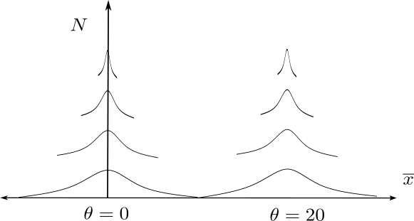
Here, we have \(\overline{x}\) in the horizontal direction, and \(N\) in the vertical direction. Strictly speaking, we have a joint distribution in this space, but I have plotted vertically spaced densities to show how the density of \(\overline{x}\) is centered at the true \(\theta\), but narrows as \(N\) increases.
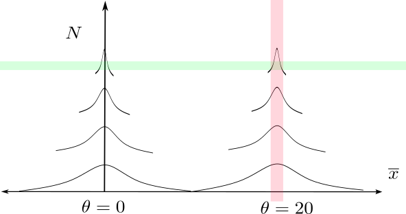
We can visualize the two censoring regions. As follows. The green censoring region, which “censors” on a particular value of \(N\), does not affect inference, because the joint probability of getting an observation in it does not depend on \(\theta\). In contrast, the probability of the red region, \(\mathcal{E}\), which corresponds to censoring a particular value of \(\overline{x}\), depends strongly on \(\theta\).
Optional stopping
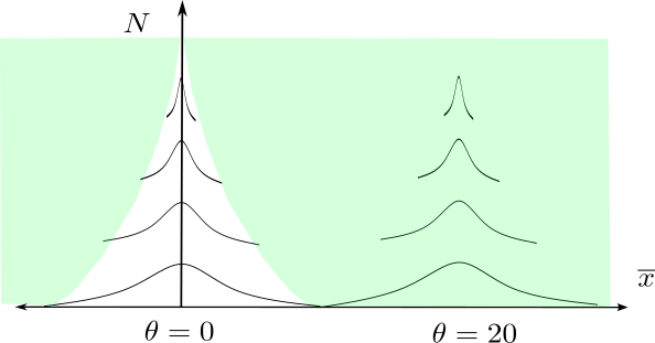
Now, we can turn to conditioning on \(\mathcal{R}\). Let’s define the optional stopping event \[ \mathcal{S}:= \{ \mathcal{x}_N \in \mathcal{R}\textrm{ and } \mathcal{x}_{N'} \notin \mathcal{R}\textrm{ for }N' < N\}. \] The event \(\mathcal{S}\) is precisely the event that \(\mathcal{x}_N\) is the first dataset in the rejection region in the sequence of datasets \((x_1)\), \((x_1, x_2)\), \((x_1, x_2, x_3)\), up to \((x_1, \ldots, x_N)\). A particular draw of \((\mathcal{x}_N, N)\) is either in \(\mathcal{S}\) or not, and we imagine only reporting datasets that are in \(\mathcal{S}\). One can see that “censoring” on the event \(\mathcal{S}\) is the same as the optional stopping rule “run until we can reject.”
But limiting to observations that are in \(\mathcal{S}\) is not really censoring in the sense that, no matter the value of \(\theta\), the probability of \(\mathcal{S}\) is one. This region is shown in the following figure. A value of \(\theta\) corresponds to a vertical set of densities. It is clear enough that, for any \(\theta \ne 0\), eventually we must get a dataset \(\mathcal{x}_N\) in \(\mathcal{S}\). For \(\theta = 0\), you need to know the law of the iterated logarithm to see that \(\mathcal{S}\) occurs eventually with probability one, but it does.
This means that the event “\(\mathcal{S}\) occurs” is ancillary for \(\theta\). Like the event \(N = 20\), it has the same probability for each \(\theta\). The likelihood describing the process of generating data differs from the likelihood for a fixed \(N\) only by an indicator that \(\mathcal{S}\) occurs, and so Bayesian inference is unchanged! \[ p(\mathcal{x}_N, N, | \mathcal{S}\textrm{ occurs}, \theta) = \frac{p(\mathcal{x}_N, N,\mathcal{S}\textrm{ occurs} | \theta)}{p(\mathcal{S}\textrm{ occurs} | \theta)} = p(\mathcal{x}_N, N, \mathcal{S}\textrm{ occurs} | \theta) = p(\mathcal{x}_N, N| \theta) 1\left( \mathcal{S}\textrm{ occurs} \right), \] where the final line follows because \(\mathcal{S}\) occurring is a measurable function of \(\mathcal{x}_N\) and \(N\).
So Bayesian inference is unchanged. But the probability of landing in \(\mathcal{R}\) given that \(\mathcal{S}\) occurs is of course now one, so the original hypothesis test needs to be modified to account for the fact that we have conditioned on this ancillary statistic. One can either call it a valid test with level \(1\) (which is useless of course), or use a wider \(q_{\alpha}\) in the rejection region \(\mathcal{R}\) than you do in the censoring region \(\mathcal{S}\). This is possible, but tedious — in contrast to the Bayesian solution, which requires no modification.
What scale of \(\theta\) do you care about?
In order to understand why this seems counterintuitive, it might help to view the rejection region on a scale where we show \(\sqrt{N} \overline{x}\) on the x-axis. In this view, which is the scale of the test statistic rather than the sample mean, the rejection region looks superficially like a “bad” region, akin to the region \(\mathcal{E}\) of censoring only when \(\overline{x}\) is close to \(20\).
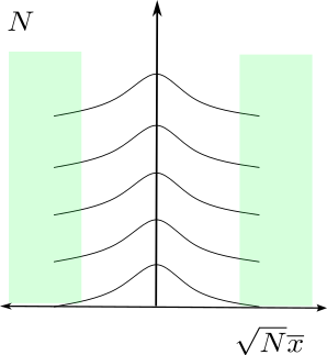
But this is misleading, because the scale of \(\theta\) changes as you move vertically in this picture. Lines of fixed \(\theta\) all curve away from the y-axis in this picture except for \(\theta = 0\). In other words, in order for it to be problematic for Bayesian inference to censor on \(\mathcal{S}\), you need to be interested in finer and finer scales oa \(\theta\) as \(N\) increases. But the Bayesian perspective places a prior on the scale of \(\theta\), not on the scale \(\sqrt{N} \theta\).
In contrast, frequentist inferece with a fixed level is in fact concerned with finer and finer scales of \(\theta\) as \(N\) increases, since we want power to increase to infinity for every alternative. This tension between Bayesian and frequentist approaches leads to the well-known disconnect between “statistical significance” and “practical signicificance” in hypothesis testing.
In fact, this picture makes clear that this stopping rule can in fact be thought of has effectively forcing you to gather more data when \(\theta\) is close to zero, and nothing more. Note that, for \(\theta\) far from \(0\), you terminate right away, whereas when you are close to \(0\), you might need to increase \(N\) before entering \(\mathcal{S}\). Coupling \(N\) and \(\theta\) might in fact make sense if you need precise estimates very close to zero, but don’t need precise estimates if it’s far away.
Conclusion
Putting this together, we can see that terminating when we land in \(\mathcal{R}\) is the same as throwing away samples that don’t land in \(\mathcal{S}\), and that the probability that we land in \(\mathcal{S}\) is independent of \(\theta\) — though it does cause us to collect more data for some \(\theta\) than for others. So it’s censoring on an ancillary statistic, and as I hope we agreed above, it shouldn’t be surprising that doing so leaves Bayesian inference unchanged, but (in general) needs to be taken into account in your frequentist rejection regions.
Berger states at the beginning of his chapter that of course we only condition on events that occur with probabilty one:
“A sequential procedure will be called proper if \(P_\theta(N < \infty) = 1\) for all \(\theta\) …. We will restrict consideration to such procedures.” - Berger (2013) 7.3
Much later, he states the the “Stopping rule principle”:
“The stopping rule … should have no effect on the final reported evidence about \(\theta\) obtained from the data.” - Berger (2013) 7.7.2
I might have phrased this “a proper stopping rule should have no effect,” since otherwise the key condition for this to be true is buried in the middle of a paragraph several pages earlier. Maybe this phrasing is what gives rise to the counterintuitive idea that Bayesian anslysis cannot be p-hacked.